Diagnosing Breast Cancer: A Machine Learning Approach

Overview

Different machine learning algorithms can behave very differently even when they are trained on the same data.

In this analysis, I compare nine supervised learning approaches for classifying breast tumors using the Wisconsin Breast Cancer Database (WBCD).

Rather than choosing a model from overall accuracy alone, I compare performance using several measures:

• sensitivity,
• specificity,
• precision,
• F1 score,
• balanced accuracy.

The models considered are:

1. Logistic Regression
2. K-Nearest Neighbors
3. Support Vector Machine
4. Naive Bayes
5. Discriminant Analysis
6. Decision Tree
7. Random Forest
8. Artificial Neural Network
9. Gradient Boosting

NoteAt a Glance

The analysis uses 699 observations and nine clinical predictors.

K-Nearest Neighbors and the Artificial Neural Network produced the highest reported F1 score and balanced accuracy in the final model comparison.

The analysis below looks not only at overall predictive performance, but also at how the methods differ in structure, tuning, sensitivity, specificity, and classification errors.

Why Breast Cancer Classification Matters

Cancer occurs when cells divide uncontrollably and may form a mass known as a tumor. Tumors may be benign or malignant.

Malignant tumors can invade surrounding tissue, so accurate identification is particularly important in applications involving cancer diagnosis.

Breast cancer remains an important public health concern, and early identification can play an important role in improving outcomes (Parkin and Fernández 2006; Ma and Jemal 2013).

Benign and malignant tumor illustration

Traditional diagnostic procedures such as mammography remain important, while statistical and machine learning techniques provide additional tools for identifying patterns associated with tumor type.

Previous studies have applied neural networks, support vector machines, and other machine learning approaches to breast cancer classification (Kiyan and Yildirim 2004; Maglogiannis et al. 2007; Sahran et al. 2008; Asri et al. 2016).

The goal of this analysis is to compare several widely used supervised learning methods under a common framework.

Data

The data come from the Wisconsin Breast Cancer Database available through the UCI Machine Learning Repository (Wolberg 1992).

The dataset contains 699 observations and nine clinical predictors measured on a scale from 1 to 10.

Variables

#	Variable	Abbreviation	Range
1	Clump Thickness	CT	1–10
2	Uniformity of Cell Size	UCSi	1–10
3	Uniformity of Cell Shape	UCSh	1–10
4	Marginal Adhesion	MA	1–10
5	Single Epithelial Cell Size	SECS	1–10
6	Bare Nuclei	BN	1–10
7	Bland Chromatin	BC	1–10
8	Normal Nucleoli	NN	1–10
9	Mitoses	—	1–10

The outcome is binary:

\[ Y = \begin{cases} 0, & \text{Benign} \\ 1, & \text{Malignant} \end{cases} \]

Treating malignant tumors as the positive class gives sensitivity a natural interpretation in this application.

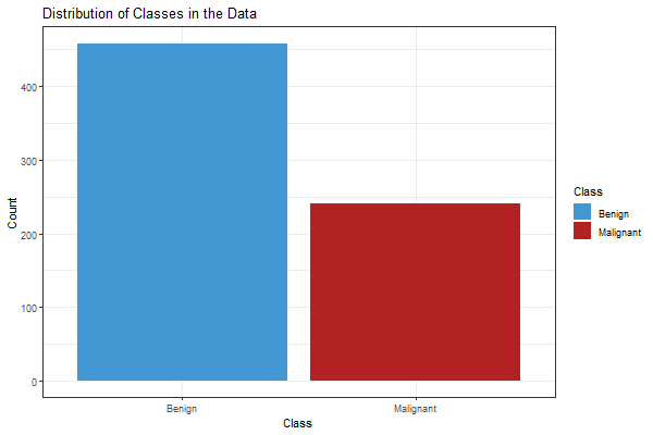
Class Distribution

The complete dataset contains:

Tumor Type	Number of Cases
Benign	458
Malignant	241
Total	699

Distribution of Classes

Train-Test Split

The observations were divided into:

\[ 80\% \text{ training} \qquad\text{and}\qquad 20\% \text{ testing} \]

The resulting samples were:

Dataset	Benign	Malignant	Total
Training	370	189	559
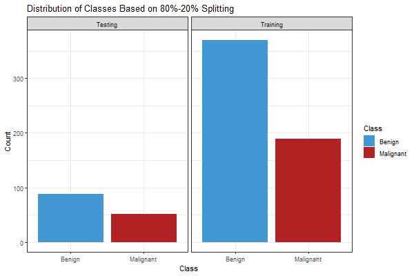
Testing	88	52	140

Distribution Based on 80%–20% Splitting

Data Preparation

library(magrittr)
library(ROCR)
library(pROC)
library(ggplot2)
library(MASS)
library(dplyr)
library(caret)
library(e1071)

data = read.table(
  file = "Breast_Cancer.txt",
  sep = ",",
  header = FALSE
)

names(data) = c(
  "id_number",
  "CT",
  "UCSi",
  "UCSh",
  "MA",
  "SECS",
  "BN",
  "BC",
  "NN",
  "Mitoses",
  "Class"
)

# Treat missing Bare Nuclei values as NA
data$BN[data$BN == "?"] = NA

# Replace missing Bare Nuclei values using the mode
val = unique(
  data$BN[
    !is.na(data$BN)
  ]
)

BN_mode = val[
  which.max(
    tabulate(
      match(
        data$BN,
        val
      )
    )
  )
]

data$BN[
  is.na(data$BN)
] = BN_mode

# Remove identification variable
data = data[, -1]

data$BN = as.numeric(
  data$BN
)

# Recode outcome:
# 0 = Benign
# 1 = Malignant

data$Class = ifelse(
  data$Class == 4,
  1,
  0
)

# Reproducible 80/20 split
set.seed(654)

train = sample(
  nrow(data),
  0.8 * nrow(data)
)

train_data = data[
  train,
]

test_data = data[
  -train,
]

Modeling and Evaluation

The models range from traditional statistical classifiers to nonlinear, tree-based, ensemble, and neural-network methods.

Because the methods differ in structure, several require parameter tuning before predictions are made on the testing data.

Cross-Validation

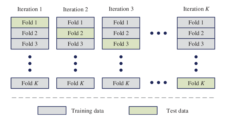
I use 10-fold cross-validation when tuning applicable models.

Let the training observations be divided into:

\[ K=10 \]

folds.

For each iteration, the model is fitted using:

\[ K-1=9 \]

folds and evaluated using the remaining fold.

The process continues until each fold has served as the validation set.

K-Fold Cross Validation

Performance Measures

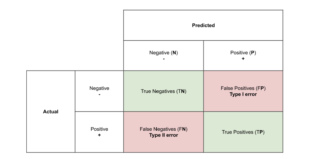
A confusion matrix can be summarized using four quantities:

Quantity	Meaning
TP	True Positive
TN	True Negative
FP	False Positive
FN	False Negative

Layout of a Confusion Matrix

Sensitivity measures the proportion of malignant tumors correctly classified:

\[ \text{Sensitivity} = \frac{TP}{TP+FN} \]

Specificity measures the proportion of benign tumors correctly classified:

\[ \text{Specificity} = \frac{TN}{TN+FP} \]

Precision measures the proportion of predicted malignant tumors that are actually malignant:

\[ \text{Precision} = \frac{TP}{TP+FP} \]

Recall is equivalent to sensitivity:

\[ \text{Recall} = \frac{TP}{TP+FN} \]

The F1 score combines precision and recall:

\[ F_1 = 2 \left( \frac{ \text{Precision}\times\text{Recall} }{ \text{Precision}+\text{Recall} } \right) \]

Balanced accuracy is the arithmetic mean of sensitivity and specificity:

\[ \text{Balanced Accuracy} = \frac{ \text{Sensitivity}+\text{Specificity} }{2} \]

Using several performance measures gives a more complete picture of classification behavior than relying on accuracy alone.

The Models

Logistic Regression

Logistic regression models the probability that an observation belongs to the malignant class.

Let:

\[ p(x) = P(Y=1\mid x) \]

Then:

\[ p(x) = \frac{ 1 }{ 1+ \exp \left[ - \left( \beta_0 + \beta_1x_1 + \cdots + \beta_px_p \right) \right] } \]

Equivalently, the log-odds can be expressed as:

\[ \log \left( \frac{ p(x) }{ 1-p(x) } \right) = \beta_0 + \beta_1x_1 + \cdots + \beta_px_p \]

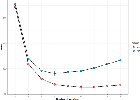
I used subset selection to compare logistic models using the Akaike Information Criterion (AIC) and Bayesian Information Criterion (BIC).

AIC and BIC Values for Subset Logistic Models

The selected predictor sets were:

Criterion	Selected Predictors
AIC	CT, UCSh, BN, BC, NN, Mitoses
BIC	CT, UCSh, BN, BC

The BIC model is more parsimonious because it retains fewer predictors.

full = glm(
  Class ~ .,
  data = train_data,
  family = binomial
)

full.prob = predict(
  full,
  test_data,
  type = "response"
)

full.pred = ifelse(
  full.prob > 0.5,
  1,
  0
)

conf.full = confusionMatrix(
  as.factor(full.pred),
  as.factor(test_data$Class),
  mode = "everything",
  positive = "1"
)

conf.full$byClass[
  c(
    "Sensitivity",
    "Specificity",
    "Balanced Accuracy"
  )
]

      Sensitivity       Specificity Balanced Accuracy 
        0.9807692         0.9545455         0.9676573 

K-Nearest Neighbors

K-Nearest Neighbors classifies a new observation according to nearby observations in the predictor space (Cover and Hart 1967).

For two observations \(x_i\) and \(x_j\), Euclidean distance is:

\[ d(x_i,x_j) = \sqrt{ \sum_{r=1}^{p} \left( x_{ir}-x_{jr} \right)^2 } \]

The basic KNN procedure is:

1. Calculate the distance between observations.
2. Find the \(K\) nearest observations.
3. Assign the majority class among those neighbors.

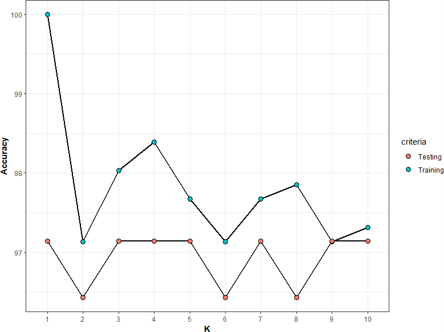
Values of \(K\) from 1 through 10 were compared.

K Values and Training/Testing Errors

The selected value was:

\[ K=9 \]

At this value, both the reported training and testing accuracies were approximately:

\[ 97.143\% \]

Support Vector Machine

A Support Vector Machine searches for a separating hyperplane with a large margin between classes (Cortes and Vapnik 1995).

For a linear classifier, a decision boundary can be written as:

\[ w^Tx+b=0 \]

Classification depends on the sign of:

\[ w^Tx+b \]

A common hard-margin formulation is:

\[ \min_{w,b} \frac{1}{2} \lVert w\rVert^2 \]

subject to:

\[ y_i(w^Tx_i+b)\geq 1 \]

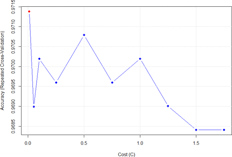
In practical applications, the cost parameter \(C\) controls the trade-off between allowing classification errors and maintaining a wider margin.

Cost Parameter Tuning for SVM

Naive Bayes

Naive Bayes is a probabilistic classifier based on Bayes’ theorem:

\[ P(A\mid B) = \frac{ P(B\mid A)P(A) }{ P(B) } \]

For classification:

\[ P(Y=k\mid X) \propto P(Y=k)P(X\mid Y=k) \]

Under the conditional independence assumption:

\[ P(X\mid Y=k) = \prod_{j=1}^{p} P(X_j\mid Y=k) \]

Therefore:

\[ P(Y=k\mid X) \propto P(Y=k) \prod_{j=1}^{p} P(X_j\mid Y=k) \]

nb.fit = naiveBayes(
  Class ~ .,
  data = train_data
)

nb.pred = predict(
  nb.fit,
  test_data
)

conf.nb = confusionMatrix(
  as.factor(nb.pred),
  as.factor(test_data$Class),
  mode = "everything",
  positive = "1"
)

conf.nb$byClass[
  c(
    "Sensitivity",
    "Specificity",
    "Balanced Accuracy"
  )
]

      Sensitivity       Specificity Balanced Accuracy 
        1.0000000         0.9204545         0.9602273 

Discriminant Analysis

I considered both Linear Discriminant Analysis (LDA) and Quadratic Discriminant Analysis (QDA).

Linear Discriminant Analysis

LDA assumes a common covariance matrix across classes.

The discriminant function can be written as:

\[ \delta_k(x) = x^T\Sigma^{-1}\mu_k - \frac{1}{2} \mu_k^T \Sigma^{-1} \mu_k + \log(\pi_k) \]

where:

• \(\mu_k\) is the class mean vector,
• \(\Sigma\) is the common covariance matrix,
• \(\pi_k\) is the prior probability of class \(k\).

Quadratic Discriminant Analysis

QDA allows each class to have a different covariance matrix.

Its discriminant function is:

\[ \delta_k(x) = -\frac{1}{2} \log|\Sigma_k| - \frac{1}{2} (x-\mu_k)^T \Sigma_k^{-1} (x-\mu_k) + \log(\pi_k) \]

lda.fit = lda(
  Class ~ .,
  data = train_data
)

lda.pred = predict(
  lda.fit,
  test_data
)$class

conf.lda = confusionMatrix(
  as.factor(lda.pred),
  as.factor(test_data$Class),
  mode = "everything",
  positive = "1"
)

conf.lda$byClass[
  c(
    "Sensitivity",
    "Specificity",
    "Balanced Accuracy"
  )
]

      Sensitivity       Specificity Balanced Accuracy 
        0.9615385         0.9545455         0.9580420 

Decision Tree

Decision trees recursively partition the predictor space into regions associated with different outcome classes (Breiman et al. 1984).

Important components include:

• root node,
• internal decision nodes,
• branches,
• terminal nodes,
• splitting,
• pruning.

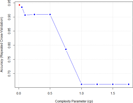
The complexity parameter \(cp\) influences tree complexity.

Complexity Parameter Tuning

The selected value was:

\[ cp=0.01 \]

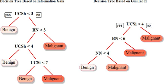
Two splitting criteria were considered.

Gini Index

For \(K\) classes, the Gini index is:

\[ G = 1- \sum_{k=1}^{K} p_k^2 \]

Entropy

Entropy is:

\[ H = - \sum_{k=1}^{K} p_k \log_2(p_k) \]

Information Gain

Information Gain measures the reduction in entropy produced by a split:

\[ IG = H(\text{parent}) - \sum_j \frac{n_j}{n} H(\text{child}_j) \]

Decision Tree Model

Random Forest

Random Forest combines predictions from many decision trees fitted to bootstrap samples.

For classification, the final prediction can be represented as a majority vote:

\[ \hat{Y} = \operatorname{mode} \left( \hat{Y}_1, \hat{Y}_2, \ldots, \hat{Y}_B \right) \]

where \(B\) is the number of trees.

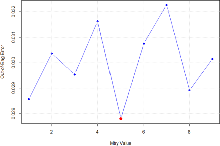
Different values of mtry were compared using out-of-bag error.

mtry Values and OOB Errors

The selected value was:

\[ mtry=5 \]

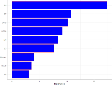
Variable Importance

Variable Importance Plot

The reported variable-importance analysis identified:

• Bare Nuclei (BN) as the most important predictor,
• Marginal Adhesion (MA) as the least important predictor according to the reported importance measure.

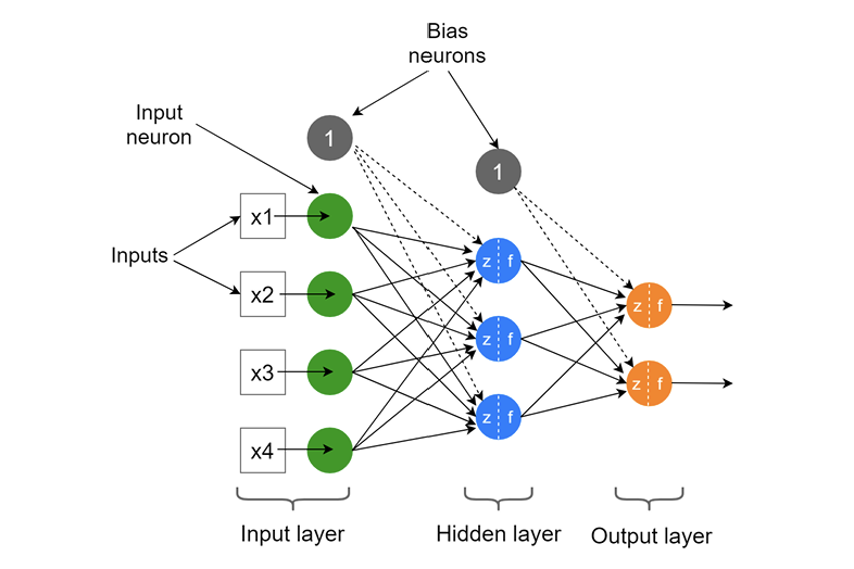
Artificial Neural Network

Artificial Neural Networks consist of interconnected units organized into layers (Rumelhart et al. 1986).

ANN Architecture

For a neuron, the weighted combination of the inputs can be expressed as:

\[ z = \beta_0 + \sum_{j=1}^{p} w_jx_j \]

The output is obtained through an activation function:

\[ a=g(z) \]

For a sigmoid activation function:

\[ g(z) = \frac{ 1 }{ 1+e^{-z} } \]

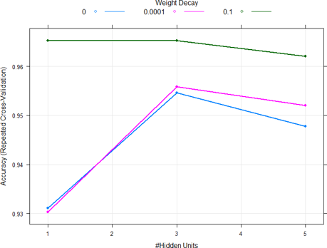
The neural network was tuned using different values for:

• number of hidden nodes,
• weight decay.

Parameter Tuning for Neural Network

The highest reported cross-validation accuracy occurred with:

Tuning Parameter	Selected Value
Hidden nodes	3
Weight decay	0.1

Thus:

\[ \text{Hidden Nodes}=3 \]

and:

\[ \text{Weight Decay}=0.1 \]

Gradient Boosting

Gradient Boosting creates an additive model sequentially, with later learners attempting to improve errors made by earlier learners.

A general representation is:

\[ F_M(x) = F_0(x) + \sum_{m=1}^{M} \nu \gamma_m h_m(x) \]

where:

• \(h_m(x)\) is the weak learner at iteration \(m\),
• \(\gamma_m\) determines the learner’s contribution,
• \(\nu\) is the shrinkage or learning-rate parameter.

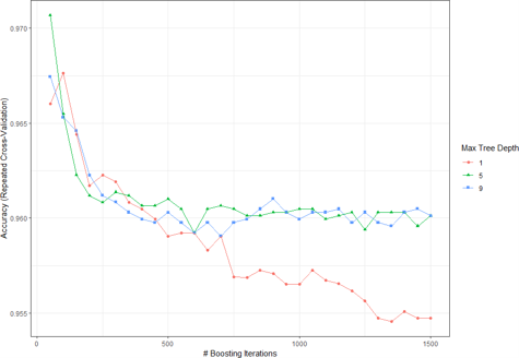
The model was tuned over:

• number of trees,
• interaction depth,
• shrinkage,
• minimum observations per node.

Gradient Boosting Tuning

The selected parameter values were:

Parameter	Selected Value
Number of trees	50
Interaction depth	5
Shrinkage	0.1
Minimum observations per node	20

Equivalently:

\[ n_{\text{trees}}=50 \]

\[ \text{interaction depth}=5 \]

\[ \text{shrinkage}=0.1 \]

\[ n_{\text{min obs in node}}=20 \]

Model Performance

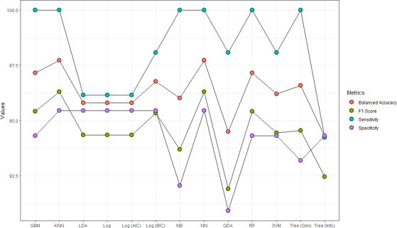
After fitting and tuning the models, I compared their test-set performance using sensitivity, specificity, F1 score, and balanced accuracy.

Performance Metrics

Performance Comparison

Method	F1 Score (%)	Sensitivity (%)	Specificity (%)	Balanced Accuracy (%)
Logistic (AIC)	94.34	96.15	95.45	95.80
Logistic (BIC)	95.33	98.08	95.45	96.77
Decision Tree (Information Gain)	92.45	94.23	94.32	94.27
Decision Tree (Gini)	94.55	100.00	93.18	96.59
K-Nearest Neighbors Selected	96.30	100.00	95.45	97.73
Support Vector Machine	94.44	98.08	94.32	96.20
Gradient Boosting	95.41	100.00	94.32	97.16
Artificial Neural Network Selected	96.30	100.00	95.45	97.73
Naive Bayes	93.69	100.00	92.05	96.02
LDA	94.34	96.15	95.45	95.80
QDA	91.89	98.08	90.91	94.49
Random Forest	95.41	100.00	94.32	97.16

Highlighted rows indicate the two models with the highest reported F1 score and balanced accuracy.

What the Results Show

Several patterns emerge from the model comparison.

Selected Models

K-Nearest Neighbors and the Artificial Neural Network produced the highest reported F1 score:

\[ F_1=96.30\% \]

and the highest reported balanced accuracy:

\[ \text{Balanced Accuracy}=97.73\% \]

Both also achieved:

\[ \text{Sensitivity}=100\% \]

and:

\[ \text{Specificity}=95.45\% \]

The final performance measures are identical, but the fitted models are very different.

Model	Selected Configuration	Test Accuracy	F1 Score	Sensitivity	Specificity	Balanced Accuracy
K-Nearest Neighbors	\(K=9\)	97.14%	96.30%	100.00%	95.45%	97.73%
Artificial Neural Network	3 hidden nodes; weight decay = 0.1	97.14%	96.30%	100.00%	95.45%	97.73%

KNN makes predictions according to nearby observations in the predictor space.

The Neural Network instead learns a nonlinear relationship between the predictors and outcome through weighted connections and hidden units.

Despite these different modeling approaches, they produced the same classifications on the testing sample.

Sensitivity Across Models

Several methods achieved:

\[ \text{Sensitivity}=100\% \]

These were:

• K-Nearest Neighbors,
• Artificial Neural Network,
• Random Forest,
• Gradient Boosting,
• Naive Bayes,
• Decision Tree using the Gini criterion.

Because malignant tumors are treated as the positive class, sensitivity is:

\[ \text{Sensitivity} = \frac{ \text{Malignant tumors correctly classified} }{ \text{Total malignant tumors} } \]

A sensitivity of 100% means that all malignant observations in the testing sample were correctly classified.

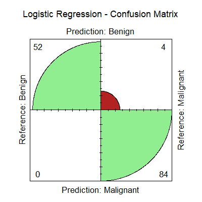
Confusion Matrix for KNN and the Neural Network

Confusion Matrix — KNN and Neural Network

Both selected models produced the same reported confusion matrix:

Actual Class	Predicted Benign	Predicted Malignant
Benign	84	4
Malignant	0	52

Therefore:

\[ TP=52 \]

\[ TN=84 \]

\[ FP=4 \]

\[ FN=0 \]

Sensitivity

Sensitivity is:

\[ \text{Sensitivity} = \frac{TP}{TP+FN} \]

Substituting the observed values:

\[ \text{Sensitivity} = \frac{52}{52+0} \]

\[ = 1.00 = 100\% \]

Thus, all 52 malignant tumors in the testing sample were correctly classified.

Specificity

Specificity is:

\[ \text{Specificity} = \frac{TN}{TN+FP} \]

Therefore:

\[ \text{Specificity} = \frac{84}{84+4} \]

\[ = 0.9545 = 95.45\% \]

Thus, 84 of the 88 benign tumors were correctly classified.

Precision

Precision is:

\[ \text{Precision} = \frac{TP}{TP+FP} \]

Therefore:

\[ \text{Precision} = \frac{52}{52+4} \]

\[ = 0.9286 = 92.86\% \]

F1 Score

The F1 score is:

\[ F_1 = 2 \left( \frac{ \text{Precision}\times\text{Recall} }{ \text{Precision}+\text{Recall} } \right) \]

Using:

\[ \text{Precision}=0.9286 \]

and:

\[ \text{Recall}=1.00 \]

gives:

\[ F_1 \approx 0.9630 = 96.30\% \]

Balanced Accuracy

Balanced accuracy is:

\[ \text{Balanced Accuracy} = \frac{ \text{Sensitivity}+\text{Specificity} }{2} \]

Therefore:

\[ \text{Balanced Accuracy} = \frac{ 100+95.45 }{2} \]

\[ = 97.725 \% \approx 97.73\% \]

Overall Accuracy

Overall accuracy is:

\[ \text{Accuracy} = \frac{ TP+TN }{ TP+TN+FP+FN } \]

Therefore:

\[ \text{Accuracy} = \frac{ 52+84 }{ 52+84+4+0 } \]

\[ = \frac{136}{140} \]

\[ = 0.9714 = 97.14\% \]

TipMain Takeaway

K-Nearest Neighbors and the Artificial Neural Network produced the strongest reported performance in this analysis.

Both correctly classified:

• all 52 malignant tumors, and
• 84 of the 88 benign tumors

in the testing sample.

Their reported performance was:

• Sensitivity: 100%
• Specificity: 95.45%
• Precision: 92.86%
• F1 score: 96.30%
• Balanced accuracy: 97.73%
• Overall accuracy: 97.14%

Although their final predictions were identical on this test sample, the two approaches reach those predictions using very different modeling structures.

Conclusion

This analysis compared nine supervised machine learning approaches using the Wisconsin Breast Cancer Database.

Several models produced strong classification results. K-Nearest Neighbors and the Artificial Neural Network produced the highest reported F1 score and balanced accuracy.

Random Forest and Gradient Boosting also performed strongly, each achieving 100% sensitivity and a balanced accuracy of 97.16%.

An interesting result is that increased model complexity did not automatically produce better test performance. KNN, a comparatively simple neighborhood-based classifier, produced the same final classifications as the tuned neural network.

The findings are specific to this dataset and train-test split. Future work could extend the analysis through:

• repeated cross-validation,
• ROC curves and AUC,
• probability calibration,
• alternative approaches for handling missing values,
• predictor-stability analysis,
• external validation using independent breast cancer datasets.

External validation would be especially important before drawing broader conclusions about performance in other populations or clinical settings.

References

Asri, Hiba, Hajar Mousannif, Hassan Al Moatassime, and Thomas Noel. 2016. “Using Machine Learning Algorithms for Breast Cancer Risk Prediction and Diagnosis.” Procedia Computer Science 83: 1064–69.

Breiman, Leo, Jerome Friedman, Charles J Stone, and Richard A Olshen. 1984. Classification and Regression Trees. CRC Press.

Cortes, Corinna, and Vladimir Vapnik. 1995. “Support-Vector Networks.” Machine Learning 20: 273–97.

Cover, Thomas, and Peter Hart. 1967. “Nearest Neighbor Pattern Classification.” IEEE Transactions on Information Theory 13 (1): 21–27.

Kiyan, Timur, and Tulay Yildirim. 2004. “Breast Cancer Diagnosis Using Statistical Neural Networks.” IU-Journal of Electrical and Electronics Engineering 4 (2): 1149–53.

Ma, Jiahong, and Ahmedin Jemal. 2013. “Breast Cancer Statistics.” Breast Cancer Metastasis and Drug Resistance, 1–18.

Maglogiannis, Ilias, Efthimios Zafiropoulos, and Ioannis Anagnostopoulos. 2007. “An Intelligent System for Automated Breast Cancer Diagnosis and Prognosis Using SVM Based Classifiers.” Applied Intelligence 30: 24–36.

Parkin, D Maxwell, and Lara MG Fernández. 2006. “Use of Statistics to Assess the Global Burden of Breast Cancer.” The Breast Journal 12: S70–80.

Rumelhart, David E, Geoffrey E Hinton, and Ronald J Williams. 1986. “Learning Representations by Back-Propagating Errors.” Nature 323: 533–36.

Sahran, Shahnorbanun, Dheeb Albashish, and Afnizanfaizal Abdullah. 2008. “Breast Cancer Diagnosis Using Genetic Algorithm and Neural Network.” International Journal of Computer Science.

Wolberg, William H. 1992. Wisconsin Breast Cancer Database. UCI Machine Learning Repository.

Asri, Hiba, Hajar Mousannif, Hassan Al Moatassime, and Thomas Noel. 2016. “Using Machine Learning Algorithms for Breast Cancer Risk Prediction and Diagnosis.” Procedia Computer Science 83: 1064–69.

Breiman, Leo, Jerome Friedman, Charles J Stone, and Richard A Olshen. 1984. Classification and Regression Trees. CRC Press.

Cortes, Corinna, and Vladimir Vapnik. 1995. “Support-Vector Networks.” Machine Learning 20: 273–97.

Cover, Thomas, and Peter Hart. 1967. “Nearest Neighbor Pattern Classification.” IEEE Transactions on Information Theory 13 (1): 21–27.

Kiyan, Timur, and Tulay Yildirim. 2004. “Breast Cancer Diagnosis Using Statistical Neural Networks.” IU-Journal of Electrical and Electronics Engineering 4 (2): 1149–53.

Ma, Jiahong, and Ahmedin Jemal. 2013. “Breast Cancer Statistics.” Breast Cancer Metastasis and Drug Resistance, 1–18.

Maglogiannis, Ilias, Efthimios Zafiropoulos, and Ioannis Anagnostopoulos. 2007. “An Intelligent System for Automated Breast Cancer Diagnosis and Prognosis Using SVM Based Classifiers.” Applied Intelligence 30: 24–36.

Parkin, D Maxwell, and Lara MG Fernández. 2006. “Use of Statistics to Assess the Global Burden of Breast Cancer.” The Breast Journal 12: S70–80.

Rumelhart, David E, Geoffrey E Hinton, and Ronald J Williams. 1986. “Learning Representations by Back-Propagating Errors.” Nature 323: 533–36.

Sahran, Shahnorbanun, Dheeb Albashish, and Afnizanfaizal Abdullah. 2008. “Breast Cancer Diagnosis Using Genetic Algorithm and Neural Network.” International Journal of Computer Science.

Wolberg, William H. 1992. Wisconsin Breast Cancer Database. UCI Machine Learning Repository.

Questions or Comments?

Have a question about the analysis, an idea to discuss, or an interest in collaborating? I'd be happy to hear from you.

Get in Touch