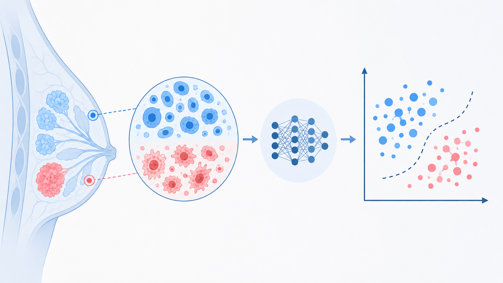
Cancer begins with uncontrolled division of cells, resulting in a visible mass called a tumor. Tumors can be either benign or malignant. Malignant tumors grow rapidly, invading and causing damage to surrounding tissues. Breast cancer is one of the most common cancers among women worldwide, representing the majority of new cancer cases and cancer-related deaths, making it a significant public health problem today (Parkin and Fernández 2006). Symptoms include breast volume changes, skin colour variations, breast pain, and genetic changes.
Benign vs Malignant Tumor
Breast cancer is the second leading cause of death among women worldwide, and more than 8% of women will develop the disease during their lifetime. The World Health Organization reports approximately 1,000,000 new diagnoses and over 500,000 deaths annually (Ma and Jemal 2013). In 2008 alone, approximately 182,460 newly diagnosed cases and 40,480 deaths were reported in the United States (Birdwell et al. 2001). Because the cause of breast cancer is still unknown, early detection is key to reducing mortality by over 40%.
Previously, mammography was the most effective detection method. Although breast cancer mortality has decreased over the past decade, expert radiologists can still miss a significant proportion of abnormalities (Birdwell et al. 2001). Machine learning (ML) has emerged as a powerful alternative, transforming qualitative diagnostic criteria into objective quantitative classification (Osareh and Shadgar 2010).
Several studies have demonstrated the effectiveness of ML for breast cancer classification. Kiyan and Yildirim achieved up to 98.8% accuracy using GRNN on WBCD (Kiyan and Yildirim 2004). Maglogiannis et al. demonstrated SVM superiority in distinguishing malignant from benign masses (Maglogiannis et al. 2007). Sahran et al. combined genetic algorithms with backpropagation neural networks, achieving 100% accuracy on clean data (Sahran et al. 2008). Asri et al. showed SVM achieves 97.13% accuracy in terms of precision and low error rate (Asri et al. 2016).
In this post, I compare nine supervised ML algorithms on the WBCD to identify the most effective approach for binary tumor classification. The methods employed are:
Logistic Regression
K-Nearest Neighbors Classifier
Support Vector Machine
Naive Bayes Classifier
Discriminant Analysis
Random Forest Classifier
Decision Tree Classifier
Artificial Neural Network
Gradient Boosting Classifier
Methods
ML provides a set of methods for identifying patterns in large databases that can then be used for prediction or decision making. It is a multidisciplinary field drawing from statistics, mathematics, and computer science. The subsections below give a brief description of each ML technique used in this project.
Logistic Regression
Logistic Regression is a classification technique that uses a logistic (sigmoid) function to model a dichotomous dependent variable, in this case, whether the tumor is benign or malignant. The sigmoid function \(y = 1/(1 + e^{-x})\) maps predicted values to probabilities between 0 and 1. A threshold parameter converts predicted probabilities into class labels: values above the threshold indicate one class, while values below indicate the other.
K-Nearest Neighbors (KNN)
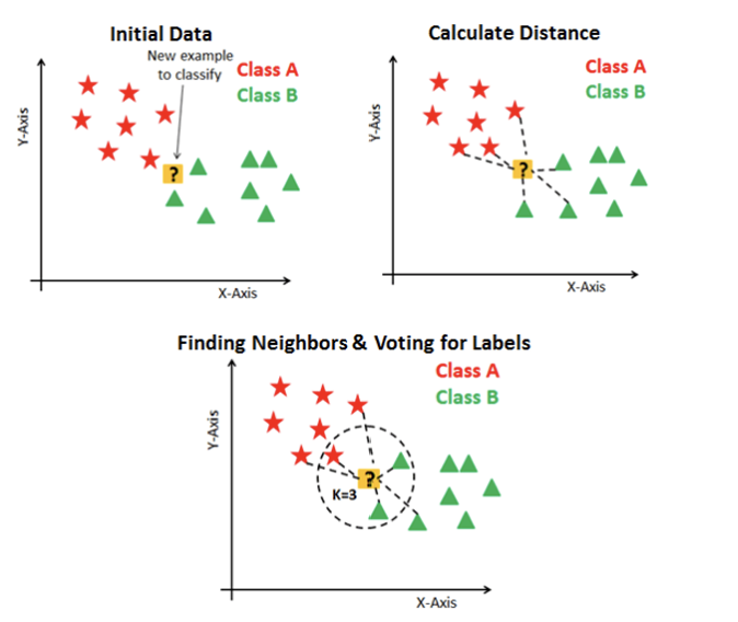
KNN is a simple algorithm that uses the entire dataset in its training phase. Whenever a prediction is required for an unseen instance, it searches through the training dataset for the K most similar instances and returns the majority class as the prediction, “if you are similar to your neighbours, then you are one of them” (Cover and Hart 1967). K is generally an odd number for binary classification. Distance measures such as Euclidean, Hamming, Manhattan, or Minkowski distance are used to find nearest neighbors. KNN has three basic steps: Calculate distance → Find closest neighbors → Vote for labels.
KNN Illustration
Support Vector Machine (SVM)
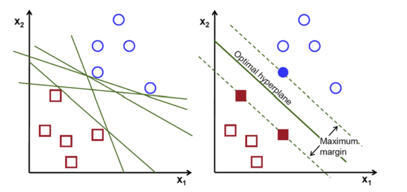
SVM is a supervised algorithm used for both classification and regression, though it is best suited for classification. The objective is to find a hyperplane in an N-dimensional space that distinctly classifies data points with the maximum margin, the maximum distance between data points of both classes (Cortes and Vapnik 1995). Maximizing the margin distance provides reinforcement so that future data points can be classified with more confidence. The dimension of the hyperplane depends on the number of features: with 2 features it is a line, with 3 features it becomes a 2-D plane.
SVM Hyperplanes
Naive Bayes
The Naive Bayes classifier is a probabilistic model based on Bayes’ theorem: \(P(A|B) = P(B|A)P(A)/P(B)\). It computes the probability of a class given the evidence. Using Bayes theorem, we can find the probability of A happening, given that B has occurred. Here, B is the evidence and A is the hypothesis. The key assumption is that predictors are conditionally independent, the presence of one feature does not affect another. Hence the term “naive.” Despite this simplification, it often performs well in practice.
Gradient Boosting
Gradient Boosting is an ensemble learning technique that combines several weak learners into a strong learner. Each predictor fits the residual errors of its predecessor rather than the original data. It has three components: a loss function (estimates model quality), weak learners (decision trees with poor accuracy), and an additive model (sequentially adds trees to reduce the loss function).
Neural Network (ANN)
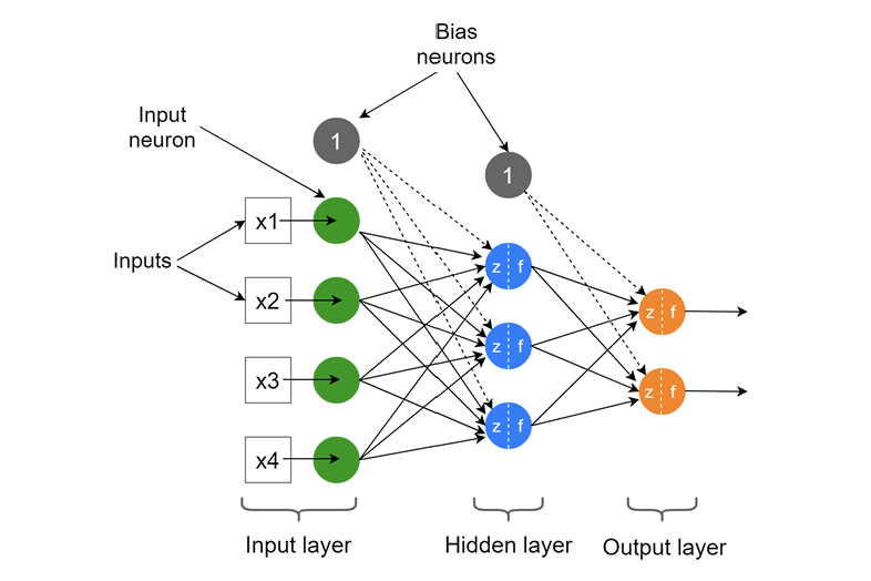
ANNs mimic the human brain’s parallel processing structure, capable of representing knowledge through pattern recognition based on past examples (Rumelhart et al. 1986). Information processing occurs at neurons connected by weighted links. Each neuron applies a nonlinear activation function to its net input to determine its output. A typical ANN consists of one input layer, one or more hidden layers, and one output layer. ANNs are superior to traditional statistical methods in recognizing high-level features and complex patterns.
ANN Architecture
Decision Tree
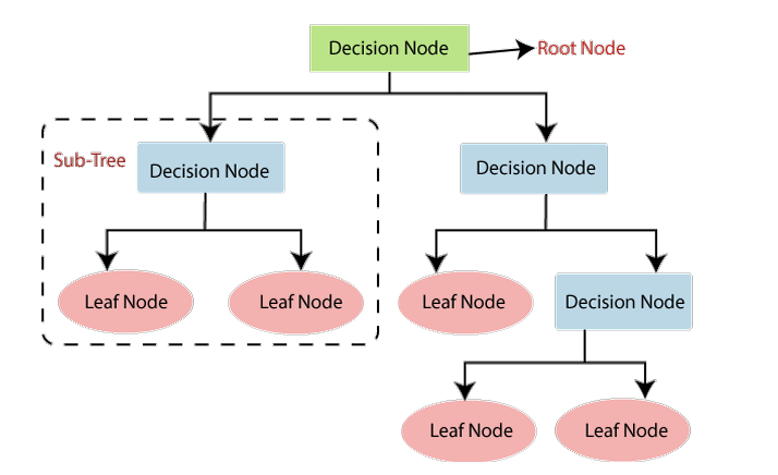
Decision Trees present classifications as a tree structure where leaves represent class labels and branches represent conjunctions of features (Breiman et al. 1984). The tree is not sensitive to noise. Key components include: Root node (represents the entire dataset), Leaf nodes (final output nodes), Splitting (dividing nodes into sub-nodes), and Pruning (removing unwanted branches). DTs are graphical representations of all possible solutions based on given conditions.
Decision Tree Architecture
Random Forest
Random Forest builds numerous decision trees using random samples with replacement, then takes a majority vote across all trees. It overcomes the overfitting problem of individual decision trees and can also assess feature importance, each variable’s value is the amount of accuracy lost by omitting it from the model.
Discriminant Analysis
Discriminant Analysis (DA) is a multivariate technique used to separate groups based on K variables and find each variable’s contribution to group separation. Linear Discriminant Analysis (LDA) assumes multivariate normality with equal covariance matrices across classes. Quadratic Discriminant Analysis (QDA) relaxes the equal covariance assumption, providing more flexibility but requiring estimation of more parameters.
Cross-Validation
Cross-validation is a crucial evaluation technique in machine learning used to evaluate the generalization ability of a model. It assesses a model’s capacity to predict new data that was not used in the estimate process in order to detect flaws like over-fitting or selection bias, as well as to predict how the model would generalize to a different data set.
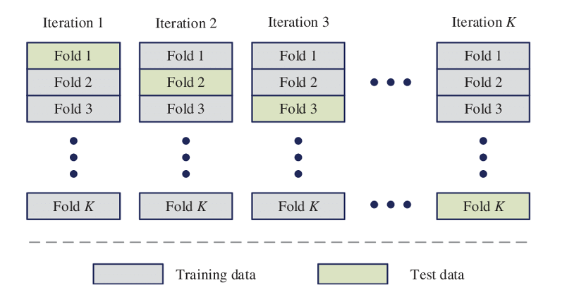
In K-fold cross-validation, the training data of size N is randomly partitioned into K equal subsets. Out of these K subsets, we use K-1 subsets as the training set and the remaining as our test set. This process is repeated for K iterations. In each iteration, a different fold is kept for testing, and the remaining K-1 is used for training. The mean of the values computed in the loop becomes the performance metric from the K-fold cross-validation. In this project, we used the 10-fold CV (i.e., setting K=10).
K-Fold Cross Validation
Performance Metrics
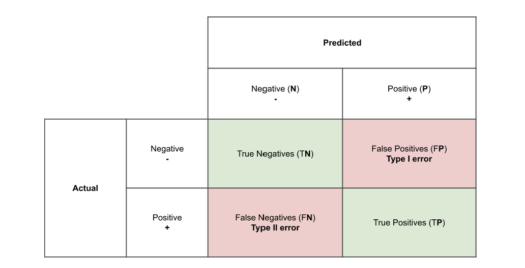
In machine learning model, we desire to know how it performs, this performance is measured with metrics. Until the performance is good enough with satisfactory metrics, the model is not worth deploying, we have to keep iterating to find the sweet spot where the model is not under-fitting nor over-fitting (a perfect balance). There are different metrics for measuring the performance of a machine learning model. The metrics used are explained below. Confusion Matrix is the way to measure the performance of a classification problem where the output can be of two or more type of classes. A confusion matrix is a table with two dimensions viz. “Actual” and “Predicted” and furthermore, both the dimensions have “True Positives”, “True Negatives”, “False Positives”, and “False Negatives”. It shows how well the model is performing, what needs to be improved, and what error it is making.
Layout of a Confusion Matrix
Where, true positive is the correctly predicted positive class outcome of the model, true negative represents the correctly predicted negative class outcome of the model, false pos¬itive is the incorrectly predicted positive class outcome of the model and false negative the incorrectly predicted negative class outcome of the model.
Sensitivity (Recall): \(TP/(TP+FN)\) — proportion of malignant cases correctly identified
Specificity: \(TN/(TN+FP)\) — proportion of benign cases correctly identified
Precision: \(TP/(TP+FP)\) — accuracy of positive predictions
F1-Score: \(2 \times (Precision \times Recall)/(Precision + Recall)\) — balance between precision and recall
Balanced Accuracy: \((Sensitivity + Specificity)/2\) — accounts for class imbalance
Analysis
Data
The data comes from the UCI Machine Learning Repository — the Wisconsin Breast Cancer Database (WBCD) (Wolberg 1992). It contains 699 observations and 9 clinical features, all rated on a scale of 1–10. The outcome is binary: Benign (1) or Malignant (0).
#
Attribute
Domain
1
Clump Thickness (CT)
1–10
2
Uniformity of Cell Size (UCSi)
1–10
3
Uniformity of Cell Shape (UCSh)
1–10
4
Marginal Adhesion (MA)
1–10
5
Single Epithelial Cell Size (SECS)
1–10
6
Bare Nuclei (BN)
1–10
7
Bland Chromatin (BC)
1–10
8
Normal Nucleoli (NN)
1–10
9
Mitoses
1–10
10
Class
0 (Benign) or 1 (Malignant)
In this data, the dependent variable (target) is the Class which is either benign or malig-nant. The other nine variables (CT, UCSi, UCSh, MA, SECS, BN, BC, NN and Mitoses) are the predictors considered in this work.
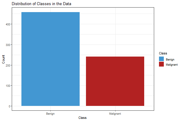
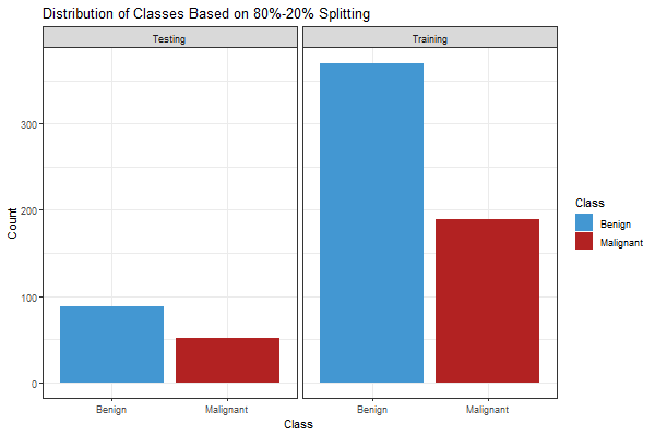
In all, the data consists of 699 instances — 458 Benign and 241 Malignant.
Distribution of Classes
To build the models, the data was split into 80% training and 20% testing. The training set has 370 Benign and 189 Malignant instances. The testing set has 88 Benign and 52 Malignant instances.
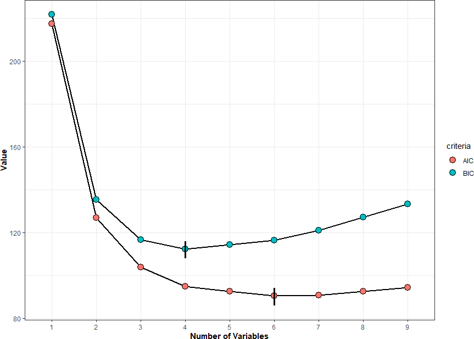
A logistic model with subset selection was built to find the optimal model, i.e., the model with predictors that are statistically significant to the prediction of breast cancer based on Akaike Information Criterion (AIC) and Bayesian Information Criterion (BIC).
AIC and BIC Values for Subset Logistic Models
full =glm(Class ~ ., data = train_data, family = binomial)full.pred = (predict(full, test_data) > .5) +0conf.full =confusionMatrix(as.factor(full.pred),as.factor(test_data$Class),mode ="everything",positive ='1')conf.full$byClass[c("Sensitivity","Specificity","Balanced Accuracy")]
The best subsets logistic model with the least AIC has 6 predictors which include CT, UCSh, BN, BC, NN and Mitoses. Also, the best subsets logistic model with the least BIC has 4 predictors which include CT, UCSh, BN and BC. Therefore, the respective predictors were considered in predicting the logistic models based on AIC and BIC.
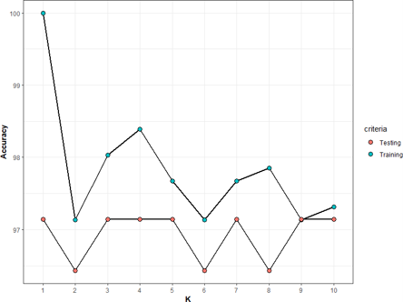
KNN Classification
Different KNN models were fitted for K from 1 to 10. To ensure that there is no issue of over-fitting, K value with a good testing accuracy and a minimal difference between the training accuracy and the testing accuracy is considered. From the Figure below, K=9 gave a high accuracy (with 97.143% training accuracy and 97.143% testing accuracy). Therefore, we used K=9 in the final prediction.
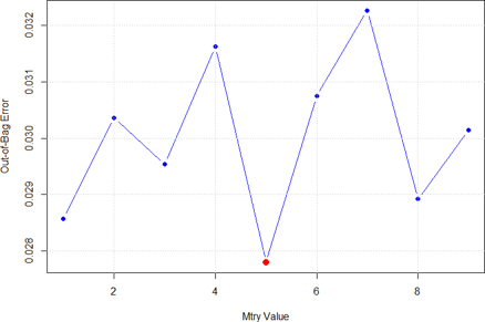
Here, we built a Random forest model from the randomForest package in R using the train data. Different “mtry” values were considered. The Out-of-Bag (OOB) error for each mtry value was evaluated.
The aim of this was to use the mtry value with the lowest OOB error (best model) to cre-ate a variable importance plot to decide on the importance of the variables and to make predictions for testing data set.
mtry Values and OOB Errors
The Figure above that the best mtry value with the least OOB error occurred at 5 (in red). Therefore, mtry=5 was used to fit a random forest model to examine its performance.
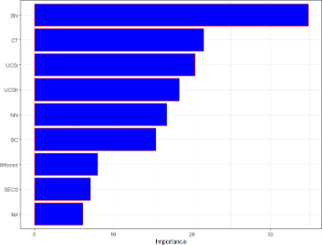
Again, the importance of the predictors were examined in the Figure below. Each value for a specific variable is the amount of accuracy lost by omitting that variable from the model. The more the accuracy declines, the more critical the variable becomes for classification success. As a result, the greater the value, the more important the variable is.
Variable Importance Plot
From the importance plot, the most important variable is BN, and the least important is MA. It ranked the variables from the most important to the least important variable. After train¬ing the random forest model and examining the importance of the variables, the predictive power of the model was tested by predicting the potential class of each instance.
Neural Network (ANN)
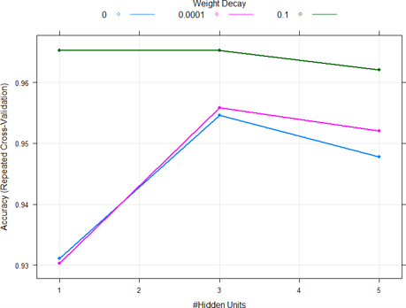
To find the optimal parameters for the neural network model, different values were consid-ered for the number of hidden nodes and the weight decay. Figure (4.7) below shows that the highest cross-validation accuracy was attained at a weight decay of 0.1 and hidden neu-rons of 3. As a result, these optimal parameters were used for predicting the testing dataset.
Parameter Tuning for Neural Network
Decision Tree
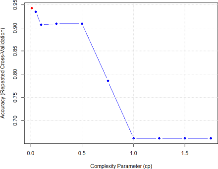
In decision tree model, the complexity parameter (cp) is a key parameter which influences the performance of the model. As a result, model tuning was performed to attain the optimal cp value with high cross-validation accuracy.
Complexity Parameter Tuning
From the Figure above, the optimal cp was achieved at 0.01 (coloured in red). As a result, this optimal parameter was used for predicting the testing dataset.
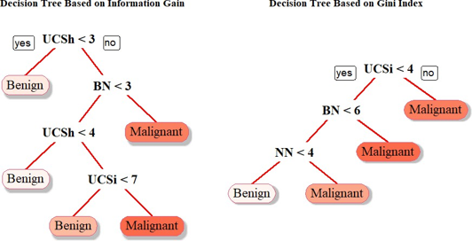
In the decision tree model, two different splitting criteria were also considered, i.e., Informa¬tion Gain and Gini Index and their respective trees are displayed below.
Decision Tree Model
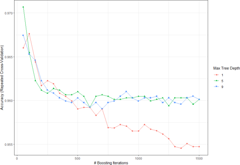
Gradient Boosting
To find the optimal parameters for the gradient boosting method, different values were con¬sidered for the number of trees, interaction.depth, shrinkage factor and the n.minobsinnode. Figure (4.11) shows that the highest cross-validation accuracy was attained at a n.trees = 50, interaction.depth = 5, shrinkage = 0.1 and n.minobsinnode = 20. As a result, these optimal parameters were used for predicting the testing dataset.
Gradient Boosting Tuning
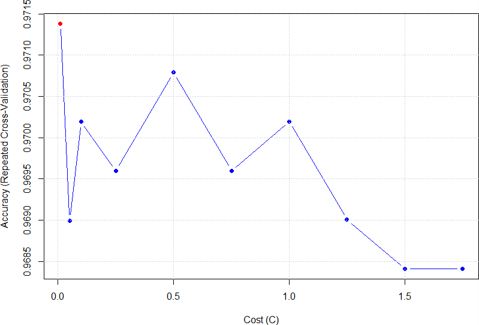
Support Vector Machine (SVM)
In this model, the cost (C) is an important parameter which influences the performance of the model. As a result, model tuning was performed to attain the optimal value with high cross-validation accuracy.
Cost Parameter Tuning for SVM
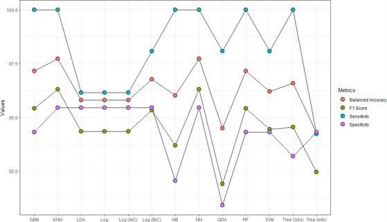
Performance Metrics Comparison
After applying the ML algorithms on the data. We used balanced accuracy, sensitivity, speci¬ficity, and F1 score to evaluate and compare the models to identify the best model.
Perfomance Metrics
Method
F1 Score (%)
Sensitivity (%)
Specificity (%)
Balanced Accuracy (%)
Logistic (AIC)
94.34
96.15
95.45
95.80
Logistic (BIC)
95.33
98.08
95.45
96.77
Decision Tree (Info)
92.45
94.23
94.32
94.27
Decision Tree (Gini)
94.55
100
93.18
96.59
K-Nearest Neighbor
96.30
100
95.45
97.73
SVM
94.44
98.08
94.32
96.20
Gradient Boosting
95.41
100
94.32
97.16
Neural Network (ANN)
96.30
100
95.45
97.73
Naive Bayes
93.69
100
92.05
96.02
LDA
94.34
96.15
95.45
95.80
QDA
91.89
98.08
90.91
94.49
Random Forest
95.41
100
94.32
97.16
: KNN and Neural Network highlighted as best performing models
Out of those that actually have the Malignant tumor, the Random Forest, KNN, Decision Tree (based on Gini Index), Neural Network, Naive-Baye’s and the Gradient Boosting perfectly classified all correctly with a sensitivity of 100%.
From the performance table, the logistic model based on AIC and BIC, KNN, neural network and LDA correctly classified a high proportion of Benign tumors out of the total Benign tu-mors in the testing data with a sensitivity value of 95.45%.
WIth regards to the F1 score and balanced accuracy, the KNN and neural network gave the same score with 96.30% (F1 score) and 97.73% (balanced accuracy). Overall, the KNN and neural network models gave the highest percentage of correct predictions.
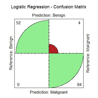
The Figure below shows the confusion matrix for the best performing models.
Confusion Matrix — Best Models (KNN and ANN)
Based on the confusion matrix for the best performing models (KNN and Neural Network), both models correctly predicted 84 Benign tumors out of 88 and perfectly classified all 52 Malignant tumors, achieving an overall correct prediction rate of 97.14%. The proportion of correctly classified Malignant tumors (Sensitivity) was 100%, while Specificity was 95.45%.
Conclusion
After comparing nine machine learning algorithms, the Neural Network (ANN) and KNN models outperformed all others, both achieving a balanced accuracy of 97.73% and F1-score of 96.30%. These models perfectly classified all malignant tumors — a critical result in a medical context where false negatives carry serious consequences. Future work should validate these findings on other breast cancer databases to confirm generalizability.
Asri, Hiba, Hajar Mousannif, Hassan Al Moatassime, and Thomas Noel. 2016. “Using Machine Learning Algorithms for Breast Cancer Risk Prediction and Diagnosis.”Procedia Computer Science 83: 1064–69.
Birdwell, Robyn L, Debra M Ikeda, Kelly F O’Shaughnessy, and Edward A Sickles. 2001. “Mammographic Characteristics of 115 Missed Cancers Later Detected with Screening Mammography.”Radiology 219 (1): 192–202.
Breiman, Leo, Jerome Friedman, Charles J Stone, and Richard A Olshen. 1984. Classification and Regression Trees. CRC Press.
Cortes, Corinna, and Vladimir Vapnik. 1995. “Support-Vector Networks.”Machine Learning 20: 273–97.
Cover, Thomas, and Peter Hart. 1967. “Nearest Neighbor Pattern Classification.”IEEE Transactions on Information Theory 13 (1): 21–27.
Kiyan, Timur, and Tulay Yildirim. 2004. “Breast Cancer Diagnosis Using Statistical Neural Networks.”IU-Journal of Electrical and Electronics Engineering 4 (2): 1149–53.
Ma, Jiahong, and Ahmedin Jemal. 2013. “Breast Cancer Statistics.”Breast Cancer Metastasis and Drug Resistance, 1–18.
Maglogiannis, Ilias, Efthimios Zafiropoulos, and Ioannis Anagnostopoulos. 2007. “An Intelligent System for Automated Breast Cancer Diagnosis and Prognosis Using SVM Based Classifiers.”Applied Intelligence 30: 24–36.
Osareh, Alireza, and Bita Shadgar. 2010. “Machine Learning Techniques to Diagnose Breast Cancer.”5th International Symposium on Health Informatics and Bioinformatics, 114–20.
Parkin, D Maxwell, and Lara MG Fernández. 2006. “Use of Statistics to Assess the Global Burden of Breast Cancer.”The Breast Journal 12: S70–80.
Rumelhart, David E, Geoffrey E Hinton, and Ronald J Williams. 1986. “Learning Representations by Back-Propagating Errors.”Nature 323: 533–36.
Sahran, Shahnorbanun, Dheeb Albashish, and Afnizanfaizal Abdullah. 2008. “Breast Cancer Diagnosis Using Genetic Algorithm and Neural Network.”International Journal of Computer Science.
Wolberg, William H. 1992. Wisconsin Breast Cancer Database. UCI Machine Learning Repository.